
Introduction
The ongoing crypto bear market has been marked by disconcerting events, to say the least, from revelations of deficient business models to exposure of outright fraudulent schemes. In this note, we step back from particular events to look at crypto price behaviors and macro indicators’ developments.
Our goal is to identify systematic patterns in crypto derivative markets and traditional spot markets. What are these indicators signaling for the current market environment? How can crypto investors make sure that they do not miss the forest for the trees?
In Section A, we propose a prediction model for the US dollar (USD), since the USD represents a timely indicator for global financing conditions, and because crypto prices tend to benefit from USD weakness and, vice versa, struggle in a macro environment where the USD is strengthening.
Sections B and C focus on the crypto derivative market and test the predictive power of BTC and ETH option prices on BTC and ETH spot prices. Section B considers call-put spread behaviors and Section C introduces the concept of “crypto risk premium” or “CRP”.
A. Growth divergences as a predictor of USD strength
As we write, the USD has started to decline vs the major DM currencies, notably the low-yielders like JPY, and also vs the Chinese CNY, following China’s “zero-covid” exit.
One driver of the recent USD’s price weakness appears to be the pricing of the peak of Fed interest rates by future bond markets. Bond futures currently forecast that the Fed policy rate will peak at ~4.84% in May 2023 and will be cut by 40bps+ in H2 2023. Admittedly, US CPI releases have surprised to the downside for the second month in a row, which can account for part of the pricing out of rate hikes.
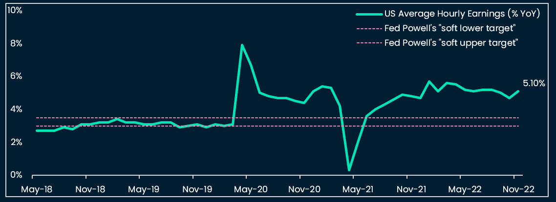
However, rate cuts or the so-called “Fed pivot” can only occur in a context of severe US macro weakness, with real growth slowing sharply. Fed Chair Powell has communicated repeatedly that 1) the risk of under-tightening outweighed the risk of over-tightening, 2) the labor market was too tight and needed rebalancing (see figure A.1). These two policy principles reinforce the necessary condition of US real growth weakness for the Fed to validate what the bond market is currently pricing. It is therefore important to understand the US real growth dynamics to assess future USD price moves.
We test the relative growth changes between the US and other countries and their predictive power on the price of the respective USD FX crosses.
To assess relative growth, we measure the changes in Purchasing Managers Indices for Manufacturing (Manufacturing PMIs) by country. Where possible we collect economists’ consensus pre-PMI publication. Where consensus is unavailable, we turn to flash surveys, which are PMI estimates released by S&P Global prior to the final releases. If forecasts or estimates are unavailable, we use the final PMI releases.
Why use Manufacturing PMIs as a proxy for growth differential shifts between countries?
- Timeliness: As surveys, PMIs have leading properties over “hard indicators” as industrial production
- Uniform methodology: The PMI calculation methodology is uniform across countries
- Auto-correlation: PMI’s declines over a certain period of time tend to be followed by further declines and vice versa for increases. This is helpful for price forecasting
- Manufacturing PMIs over Services PMIs: we use Manufacturing over Services PMI because of their superior data availability, over time and across countries
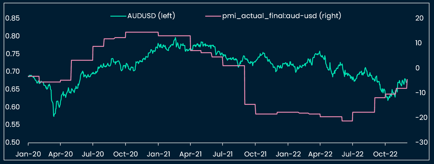
For each country's PMI, we measure the prints above 50 as positive e.g. +51 = 1 point, and the below-50 numbers as negative e.g 48 = -2. This follows the PMI’s methodology where below-50 data signal contracting activity and above-50 data expanding activity. We then measure the cross-country difference: for example if Australia expands by 1 point and the US contracts by 2 points at month M, our indicator will indicate +1-(-2)=3 points in favor of AUDUSD.
We test the indicators over the largest time samples allowed by PMI availability. The robustness of this statistical test is supported by: testing over several time periods, testing for several countries and currencies, and the absence of threshold optimization e.g. we just use the latest monthly PMIs.
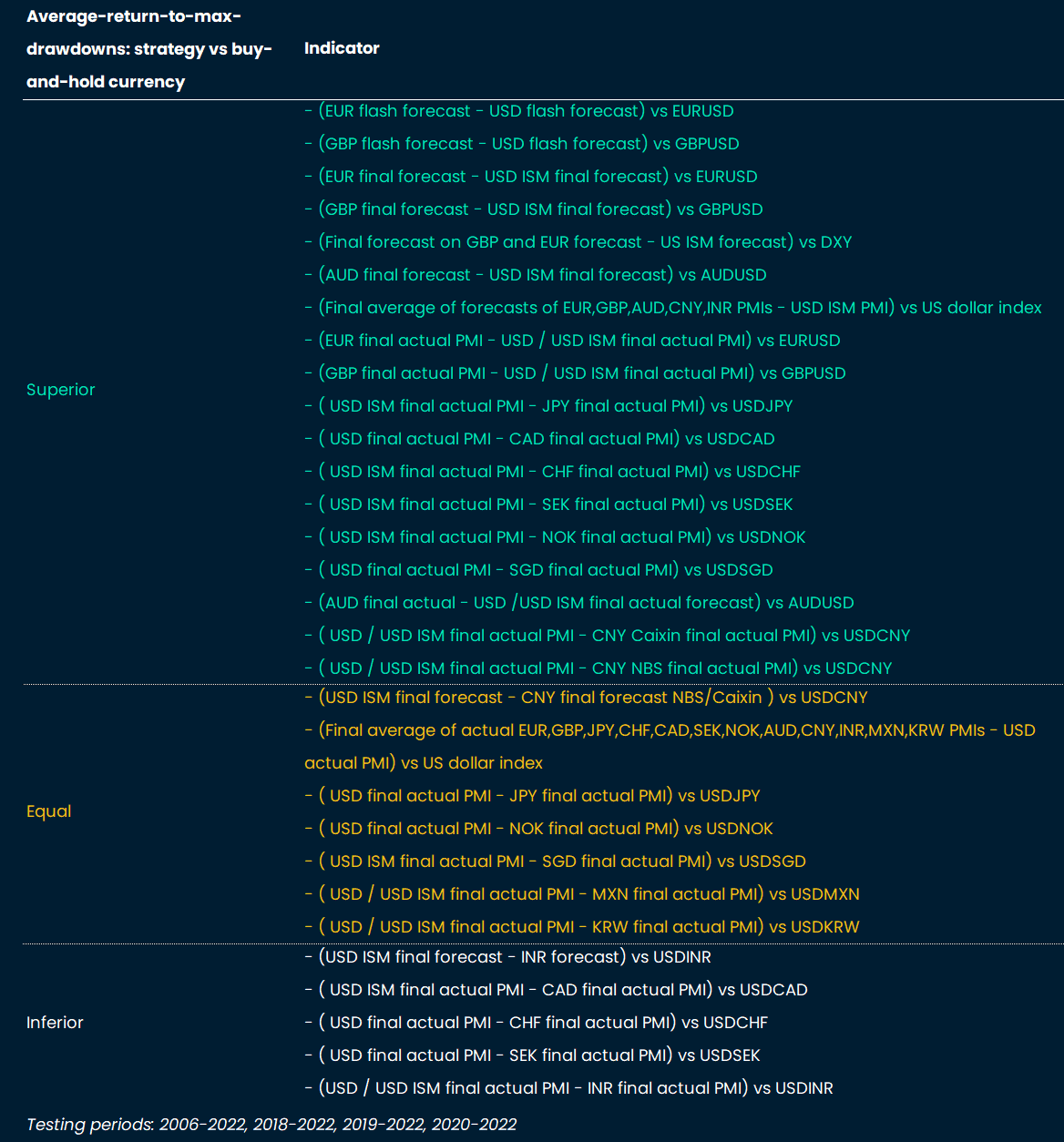
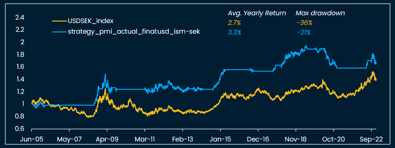
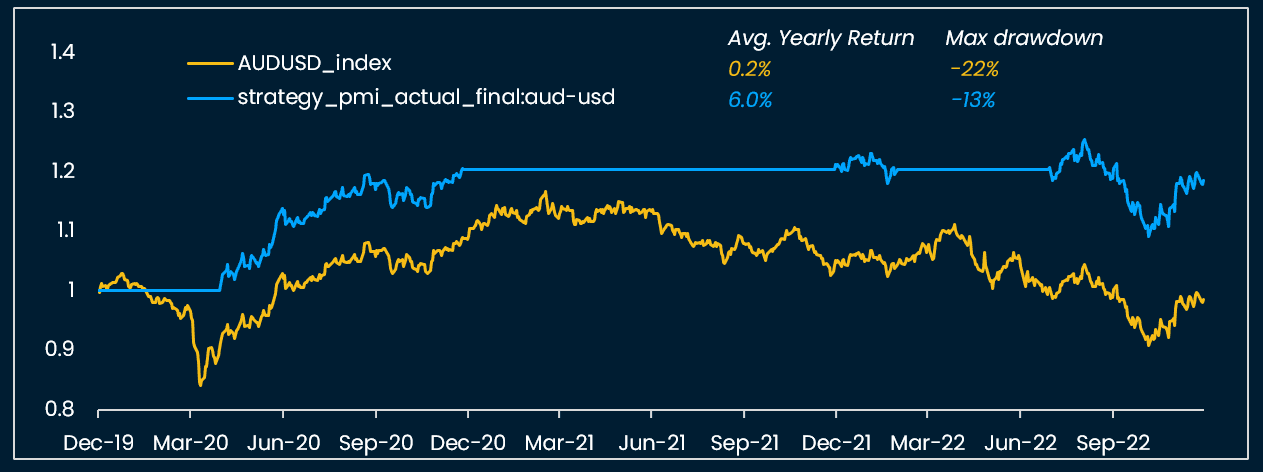
Below is a summary of the results of a simple test: whether using the PMI indicator to buy / neutralize a certain currency would have led to better risk-adjusted (return-to-max-drawdown) results than holding the currency over the same period of time.
We find that:
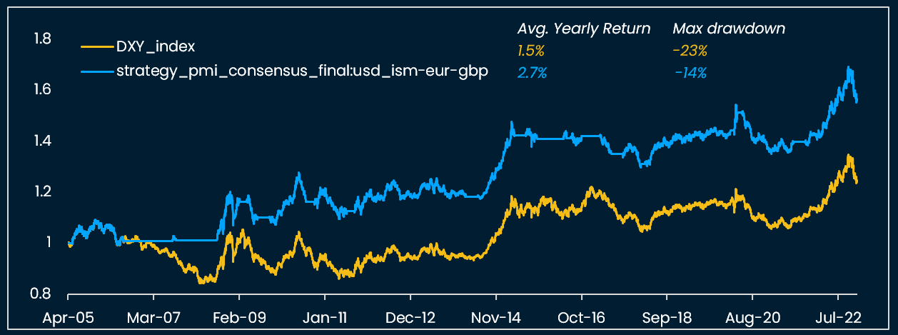
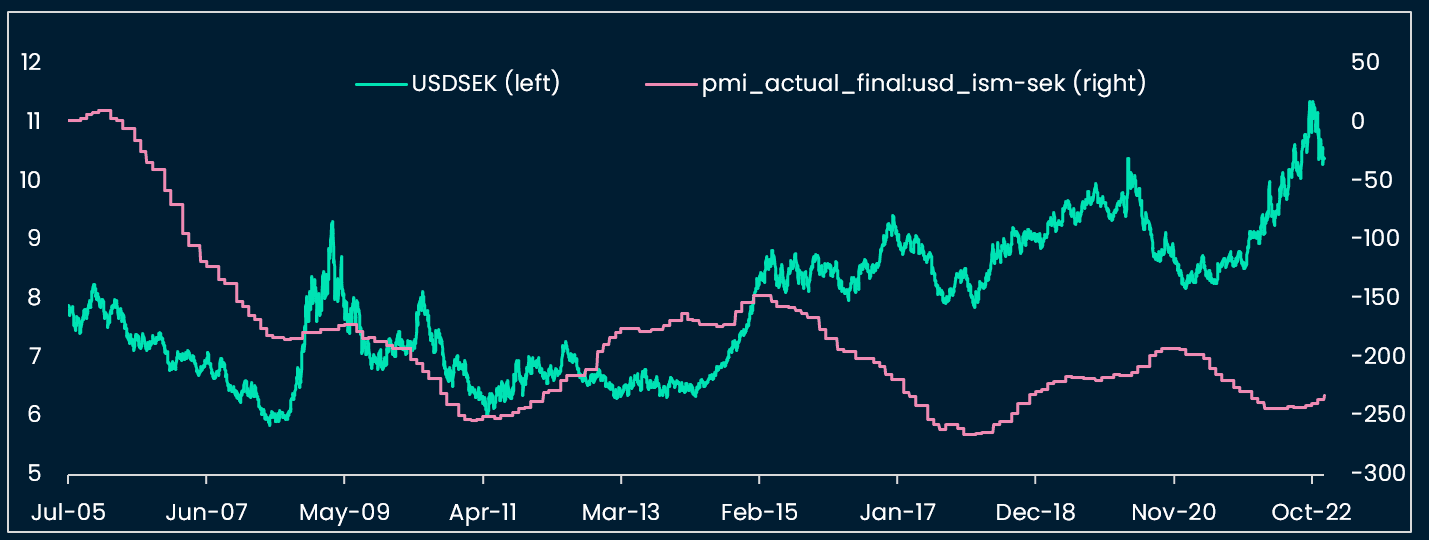
- The majority of PMI indicators, as inputs to invest in an overweight/neutral FX strategy, lead to superior results than a simple buy-and-hold strategy (see figure A.2). The PMI indicators are especially useful in capturing long-term growth divergences between two countries (see figures A.3 to A.8)
- Taking the flash or the estimate of economists delivers a slightly better performance than using actual PMIs as inputs
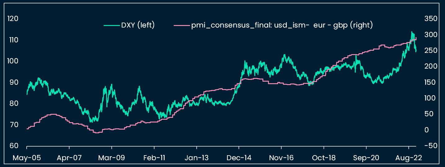
- For an approximation of the US dollar, we find that using a simple differential between the consensus for USD ISM, and a weighted EUR and GBP PMI yields the best historical performance (EURUSD and GBPUSD account for ~70% of the DXY basket, see figures A.3 and A.4) in forecasting the DXY
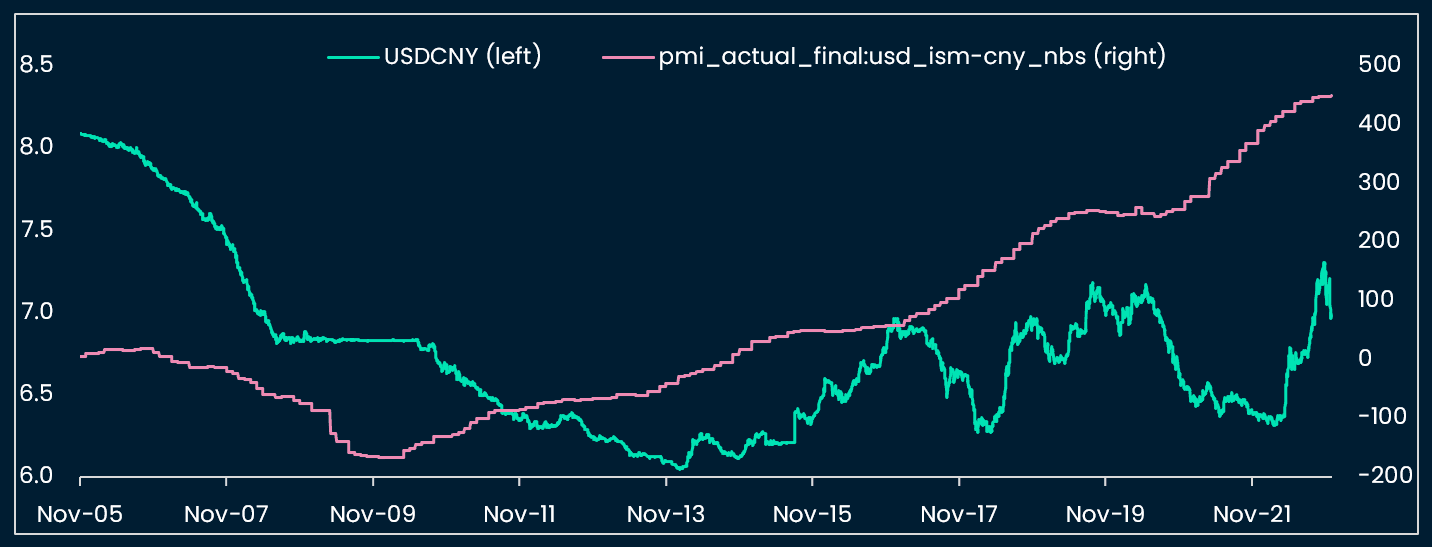
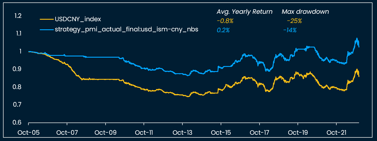
- The PMI indicators’ performance is inferior when used to forecast EM currencies: USDCNY (see figures A.9 and A.10) but especially USDKRW, USDINR, and USDMXN
Finally, the tested PMI indicators do not validate the DXY’s peaking. It follows that it is probably too early to call for a transition to easier global financial conditions, and therefore that the fundamental case for the bottoming of crypto assets is likely not there yet.
B. Call-put spread for tactical crypto investment
We turn our attention from macro indicators to the derivative markets to assess whether crypto option investors have “capitulated” yet in this bear market. To address this question we calculate the open-interest-weighted implied volatility of call vs put options or “CPIV” (call-put implied volatility) for BTC and ETH.
The literature on the relationship between equity CPIV and equity prices is mixed, with some studies arguing that CPIV in a market dominated by retail investors tends to be contrarian e.g. the higher the CPIV the lower the prospective returns of the equity underlying, but that CPIV is leading the underlying price in a market led by “professional” investors (see Doran, James and Fodor, Andy and Jiang, Danling, Call-Put Implied Volatility Spreads and Option Returns (June 21, 2013).
For our crypto CPIV study, we use historical implied volatility of BTC and ETH puts and calls sourced from Deribit via Tardis and Nansen-Query.
To create our CPIV crypto indicator, we filter out null bid prices, and group call-put open-interest-weight-ivol data by expiry range (0-10d, 11-40d, 40-90d, 91d+) and by strike range.
We decide against looking for fixed mean-regression thresholds: our data cover Jan 2021 - Nov 2022, or the end of a crypto bull market and a bear market. We assume that the derivative market is bound to evolve in future cycles and therefore test rolling percentiles for entry and exit thresholds instead.
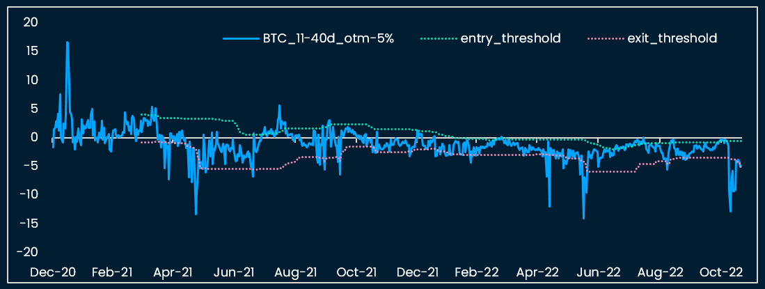
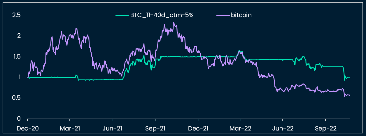
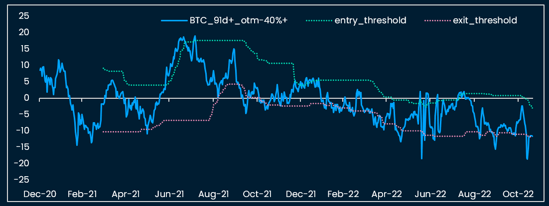
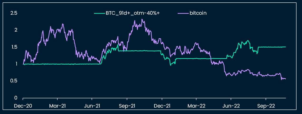
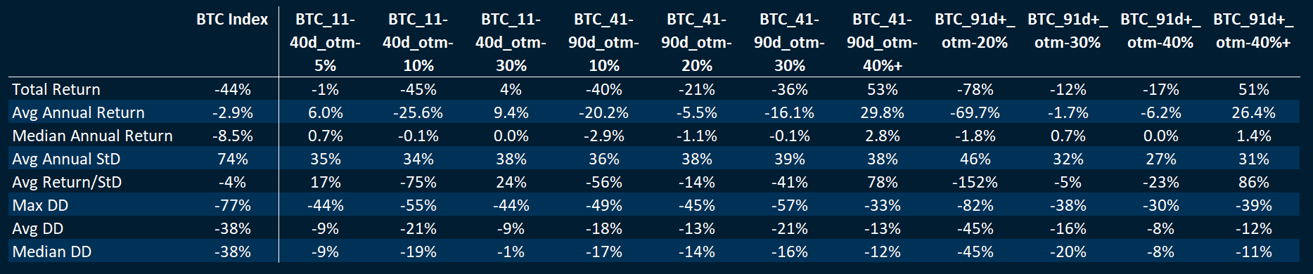
Looking at a three-month trailing 90th-percentile entry threshold (e.g. buy BTC underlying when the respective CPIV crosses below the entry threshold) and a three-month trailing 10th-percentile exit threshold (e.g. neutralize BTC underlying when the respective CPIV crosses above the exit threshold), we find that nine of the 11 indicators tested (CPIV combinations of strike ranges and maturity ranges) beat a buy-and-hold strategy in terms of total return and max drawdown, of which four significantly outperform (see figure B.9, and B.1-B.6).
Testing an entry threshold of 90th (90th percentile) or 95th, and an exit threshold equal to the 10th or 5th percentile, over a three-month or six-month period does not impact results significantly, which is encouraging when assessing the robustness of this approach.
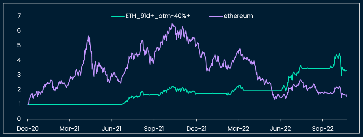
However, the strategy does not work as well for ETH options: out of 11 variations, only one beats a buy-and-hold ETH spot strategy (see figures B.7 and B.8).
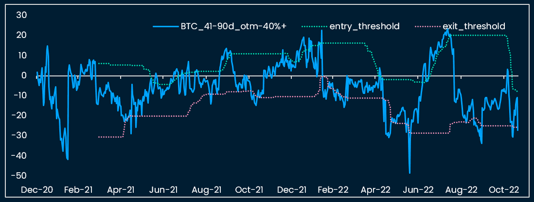
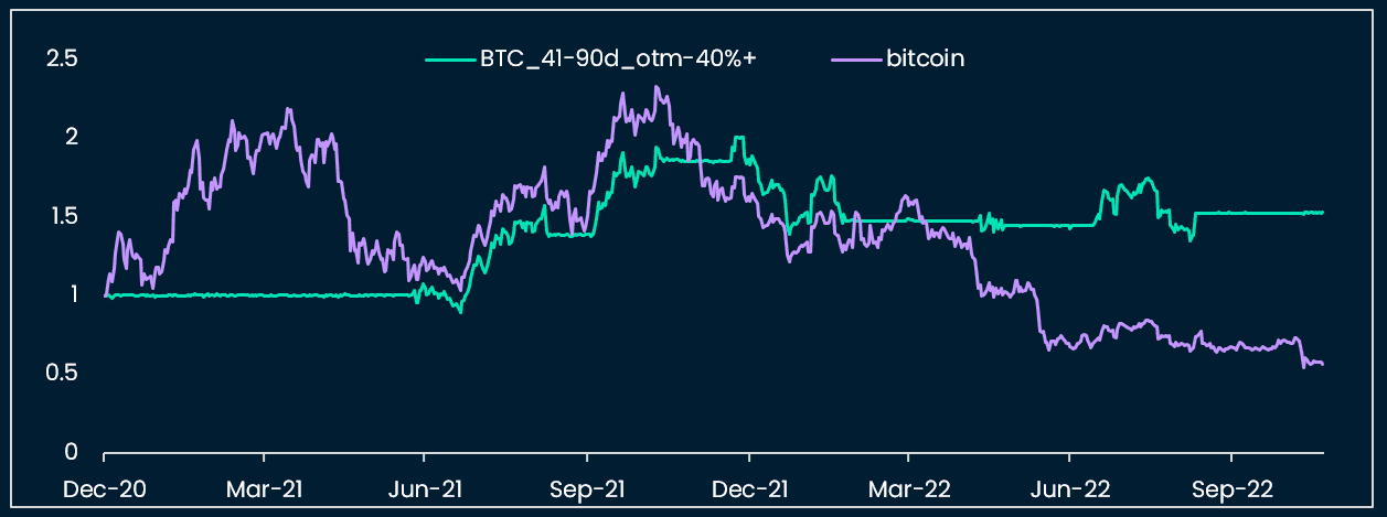
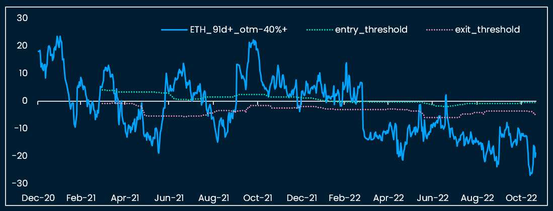
What about the behavior of derivative investors when compared to on-chain flows? We benchmark the best-performing CPIV indicator (BTC CPIV, 41-90d expiry 40% out-of-the-money) with Nansen Smart Money stablecoin risk appetite indicator (see figures B.10 and B.11).
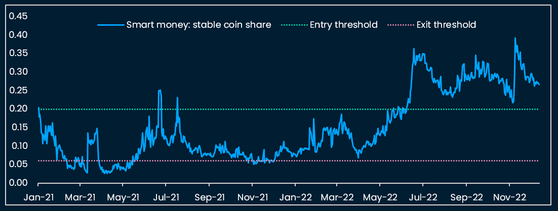
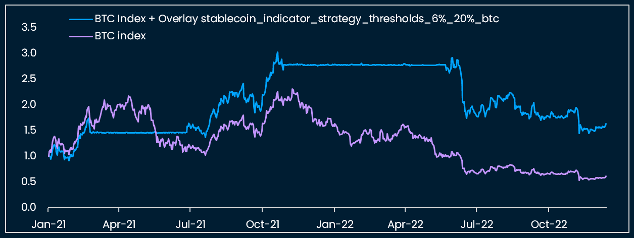
We observe that:
- The CPIV indicator generated more frequent risk-on / risk-off signals than the stablecoin indicator
- Both indicators flagged the multi-month BTC price drawdown that started in November 2021
- The stablecoin indicator returned to risk-on as early as May 2022, while the CPIV indicator was still flashing a tactical “risk-off” as of 20 November 2022
C. Crypto Risk Premium or a derivative-based valuation model for crypto
In this section we conceptualize and calculate a first version of risk premium for crypto, the “Crypto Risk Premium” or “CRP”. The risk premium, or the excess return required by investors to compensate for holding “risky assets” is linked to the perceived fundamental value of these assets by investors.
Satisfactory crypto valuation models have so far been lacking. By calculating a risk premium for BTC and ETH, we attempt to estimate the perceived value of the two assets by investors, e.g. how much premium compensation do investors require for those assets. We examine how this premium has evolved over the time sample of January 2021 to November 2022, and how it relates to the risk premium demanded by equity investors.
We make once more use of the Deribit historical option data relayed by Tardis on Nansen-Query, this time considering the intra-day bid and ask prices of calls and puts on BTC, ETH, and SOL (the time sample is much smaller for the latter, and we do not study it statistically but present a simple visualization).
We adopt the methodology developed by Ian Martin in his paper titled “What is the Expected Return on the Market?” published in April 2015. The paper presents an estimate of the Equity Risk Premium (ERP) by linking it to a measure of implied volatility, the SVIX. The advantages of using implied volatility over a more fundamental calculation (like earning yield or dividend yield forecasts for equities) are the timeliness of the data, and the minimum amount of assumptions required to estimate future yields or other inputs.
Calculating a SVIX estimate based on crypto option prices to come up with a “Crypto Risk Premium” or CRP offers the same advantages. Plus, as written above, it has so far proven difficult to generate a robust “fundamental valuation” model for crypto.
The caveats of importing the SVIX methodology from equities to crypto are that it is implicitly assumed that implied volatility for the one asset class shares close similarities with implied volatility of the other asset class. The crypto derivative market is still young and not yet as thoroughly studied as the equity option market. Therefore, it is appropriate to keep an open mind when analyzing CRP estimates. We will also compare CRP and ERP dynamics later in this note.
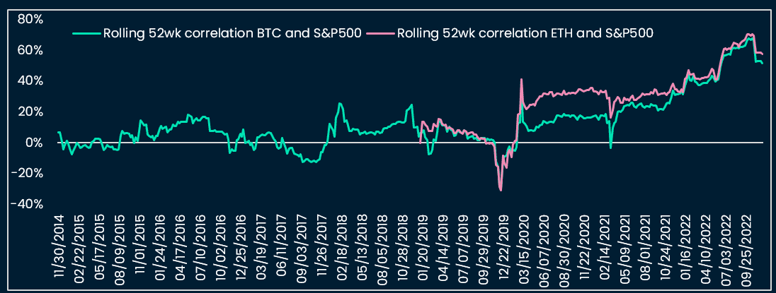
One argument for bringing equity and crypto valuation models together though is the increasing correlation between the two asset prices, especially since 2021 (see Figure C.1). One could argue that equities and crypto asset prices move together, especially during periods of risk asset sell-offs.
To calculate the SVIX for crypto, we use intra-day mid option prices as inputs to the formula presented in figure C.2. The visual representation of the SVIX estimate at a time t is drawn in figure C.3. Each daily SVIX estimate corresponds to the graphical area under the curve, refreshed at a daily frequency.
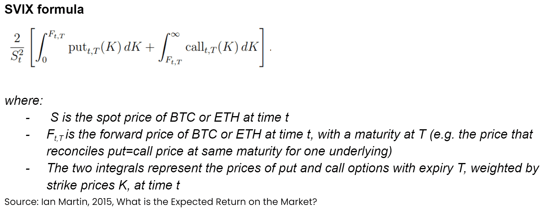
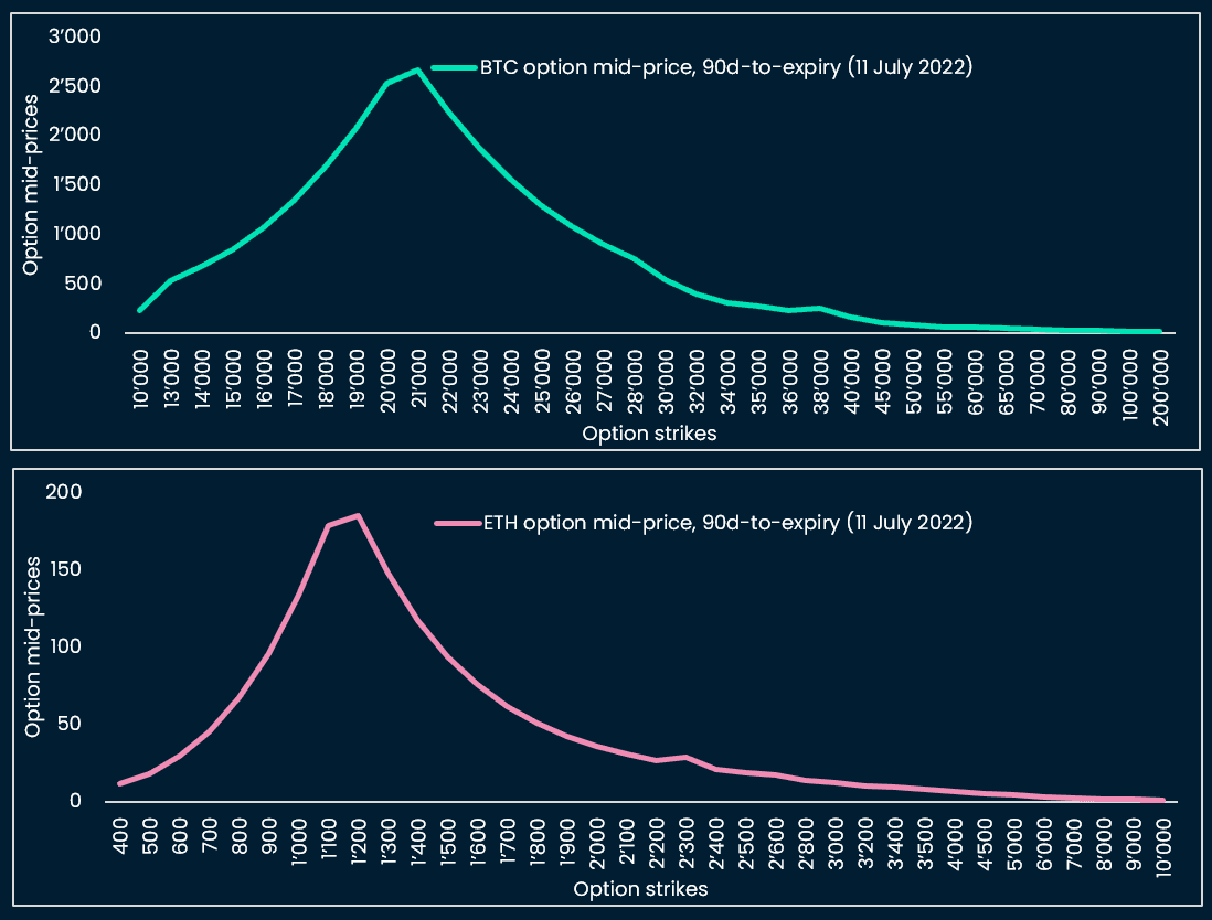
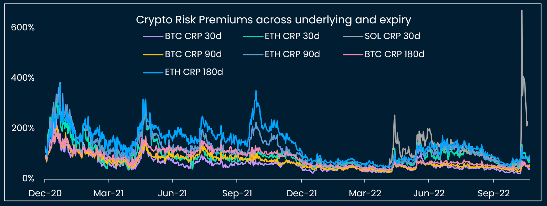
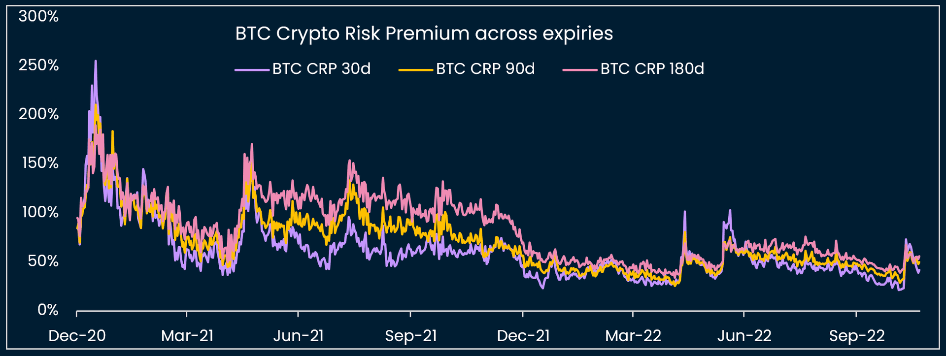
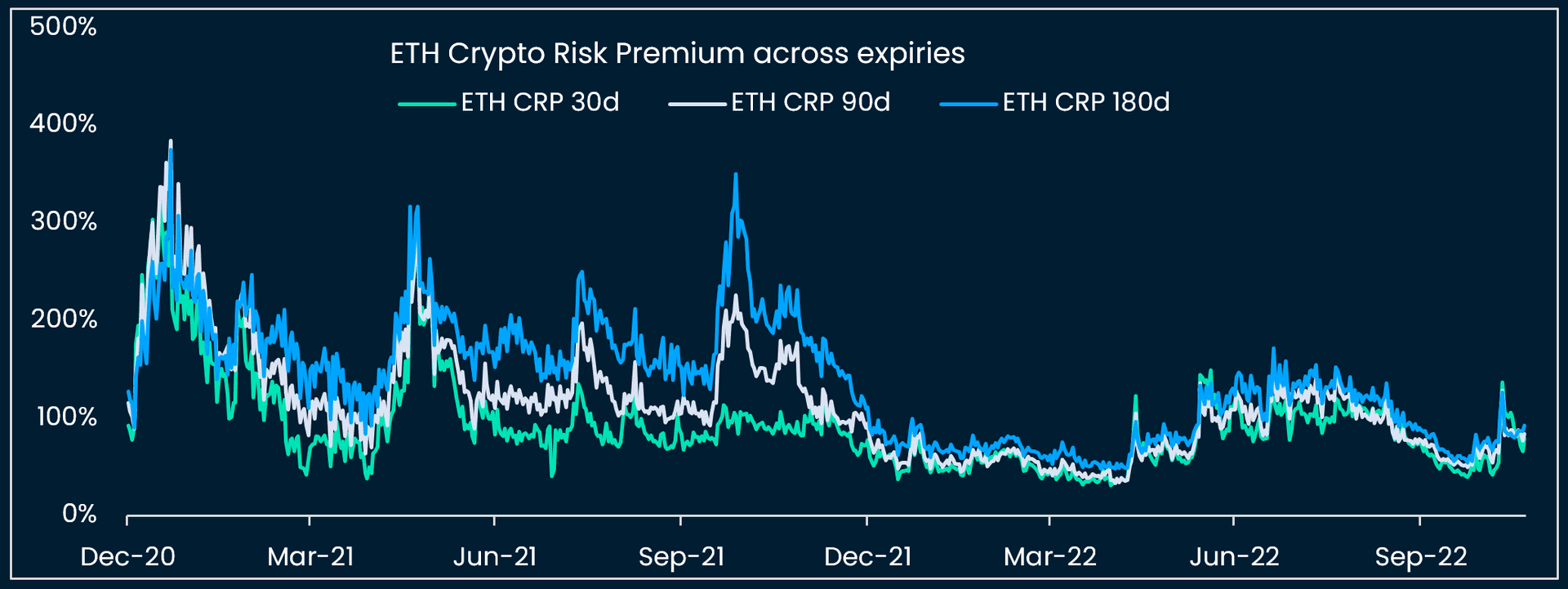
Figure C.4 charts the graphs for crypto CRPs by underlying (BTC, ETH, SOL) using options with time-to-expiration variations of 30d, 90d and 180d. A few observations:
- CRPs, regardless of underlying type or time-to-expiration, appear to be moving together
- Over time SOL CRP > ETH CRP > BTC CRP. This makes sense as it follows the hierarchy of risk observed in realized volatility
- The SVIX / CRP lines tend to surge at select points in time and then regress to more stable levels for longer periods (see figures C.5 and C.6)
- Two notable CRP surges occurred during January 2021 and May 2021 (the latter coincides with the timeline of China announcing measures to crackdown on domestic crypto mining and trading)
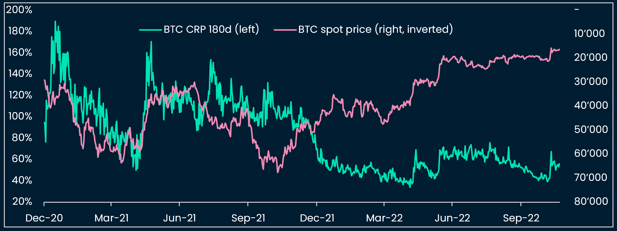
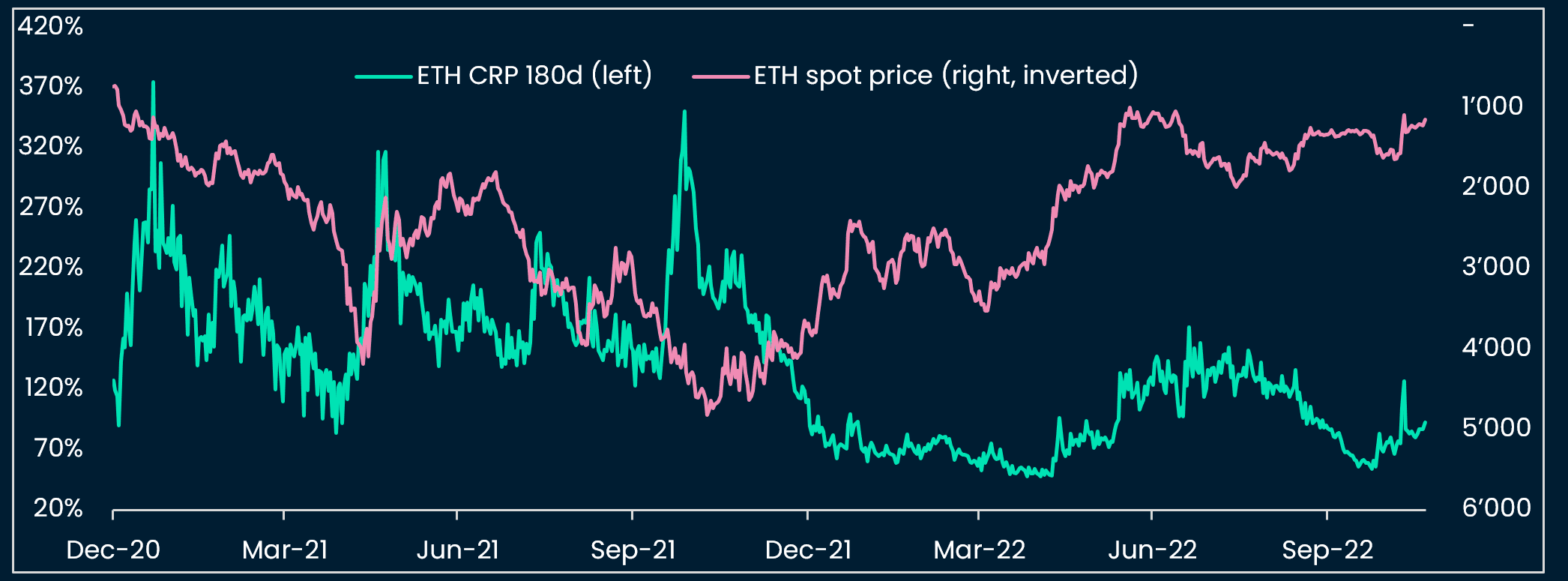
Figures C.7 and C.8 illustrate that underlying crypto prices tend to decrease when the CRP is low and jumping, and tend to increase when the CRP is high and falling.
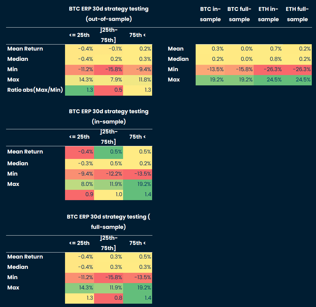
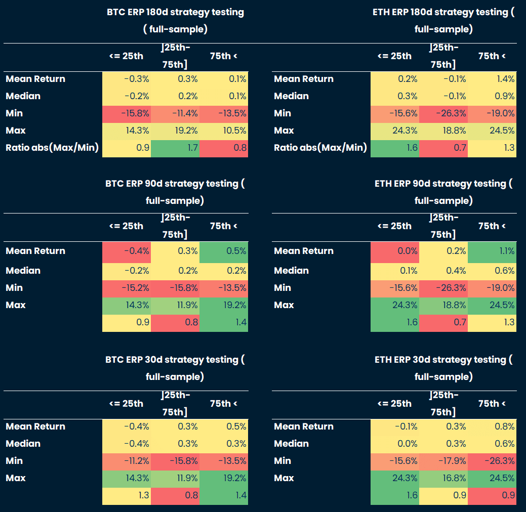
To test this observation, we calculate crypto spot performance after the CRP has reached a high vs low historical percentile. January 2021 to November 2021, or half of the time sample, is used to test various percentile thresholds in-sample.
The strategy invests in the underlying asset, here BTC, when the CRP crosses the “high” threshold and goes neutral when the CRP crosses the “low” threshold. A “high” CRP percentile threshold of 75% and “low” threshold of 25% are selected in-sample, and deliver good results out-of-sample (see Figure C.9).
We finally return to our cross-asset view and ask: How do CRP (Crypto Risk Premium) and ERP (Equity Risk Premium) compare over time?
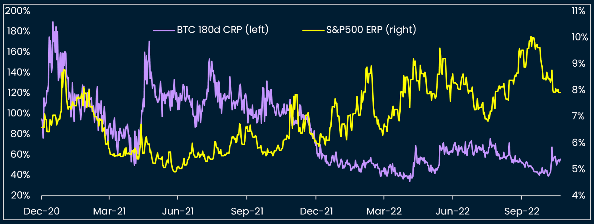
Figures C.11, C.12, C.13 and C.14 reveal that:
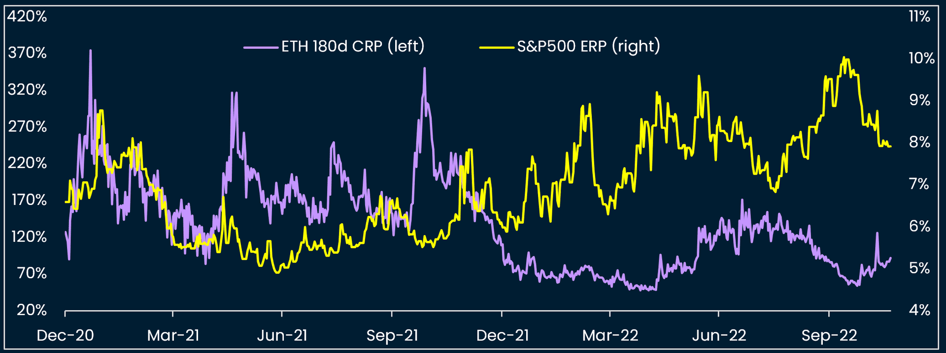
- The S&P 500 risk premium has been steadily increasing from January 2021 on
- In contrast, BTC’s and ETH’s respective CRPs have both been unstable in 2021 but have become more range-bound in 2022, even through the May 2022 UST collapse and contagion
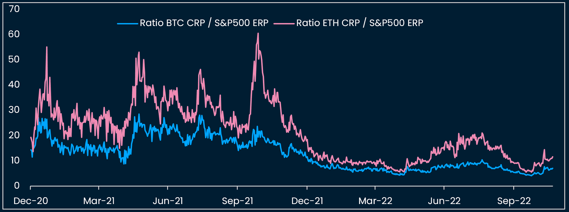
- The ratio between CRP and ERP is therefore not stable, oscillating between ~4 and ~30 for BTC relative to the S&P 500 and from ~6 to ~60 for ETH, with respective medians close to ~12 and ~20 respectively (between January 2021 and November 2022)
- The ratios between CRPs and ERP are close to the lows of the time sample as of 20 November 2022 (our last datapoint) at 7 for BTC vs S&P 500 and 12 for ETH vs S&P 500. This tends to indicate that the relative premium asked for investing in crypto vs equities has come down
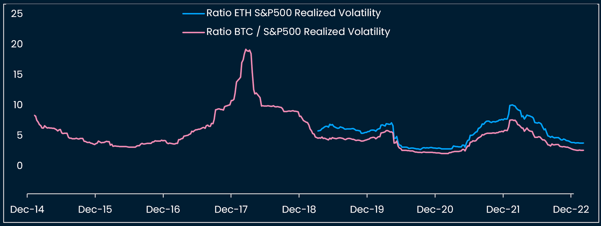
- Zooming out to a longer time sample and considering the ratio of realized volatility of BTC vs S&P 500 in figure C.15, we observe that this ratio also oscillates between 2 and 20, with a median of 5, very close to the CRP / ERP median in our sample, and also close to the latest CRP / ERP ratio
- The realized volatility ratio between BTC and the S&P 500 oscillates around ~5 with intermediary periods of sharp jumps e.g. end of 2017-January 2021, February 2020 (pandemic sell-off), and May - November 2021 (start of the more recent bear market)
To conclude on this cross-asset analysis, it seems that the relation between crypto risk premium and equity risk premium seems to have “normalized” in 2022 after an unstable 2021. What does it imply for crypto prices going forward?
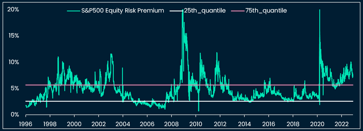
If we look at a long history of the S&P 500’s ERP (since the 1990s), we find that the ERP is relatively elevated at the moment (above its 75th historical percentile, see figure C.15), which means that equity investors are asking for a historically higher premium. However, the S&P 500’s latest ERP, which we estimate at ~8-9%, pales in comparison with the levels reached during prior recessionary market crashes: the ERP crossed above 20% in 2020 and 2008 before reversing sharply.
We therefore speculate that in the eventuality of a US recession and US equity sell-off (our main scenario for 2023 given the Fed’s determination to maintain tight financing conditions for longer), the ERP is likely to go much higher, and conversely, the CRP or crypto risk premium will probably also jump. It is therefore possible that crypto prices experience a further (and “last” ?) leg down in this cycle before financing conditions turn more favorable to both equity and crypto assets.